Hans Walser, [20130706]
Geometric Sequence and Triangles
Motivation: M. N. D., N.
1 About
Let a, b, c the sides of a triangle ABC such that ![]() (in this order)
is a geometric sequence. This means that we have a ratio r such that
(in this order)
is a geometric sequence. This means that we have a ratio r such that
![]() .
.
Figure 1 gives an example with the ratio r = 1.2.
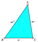
Fig. 1: Ratio r = 1.2
We will see that the Golden Section plays an important role in special cases of these triangles.
2 Special triangles
2.1 Equilateral triangle
In the trivial case of r = 1 we have the equilateral triangle (Fig. 2).
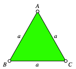
Fig. 2: Equilateral triangle
2.2 Right triangles
For r > 1 we have a < b < c. The theorem of Pythagoras yields:

The
Golden Section ![]() comes in (Walser 2001 and Walser 2013). We
get the large Right Golden Triangle of Figure 3.
comes in (Walser 2001 and Walser 2013). We
get the large Right Golden Triangle of Figure 3.
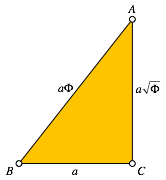
Fig. 3: Large Right Golden Triangle
For r < 1 we have a > b > c. The theorem of Pythagoras yields in this case:

We get the small Right Golden Triangle (Fig. 4).

Fig. 4: Small Right Golden Triangle
The small Golden Triangle fits into the large Golden Triangle (Fig. 5). It has the same shape like the large Right Golden Triangle, but a different orientation.
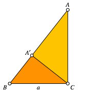
Fig. 5: Both Right Golden triangles
3 General
3.1 Range of the ratio r
The triangle inequality gives the condition a + b > c. Hence

On the other side we have a < b + c. That means

Therefore
we have the range ![]() .
.
Note that the ratios of the small Right Golden Triangle, the equilateral triangle, and the large Right Golden Triangle are within this range:
![]()
Together with the range bounds they are a geometric sequence.
3.2 Two fix points
For the general triangle we let two of the three vertices of the triangle fix and study the locus of the third point. There are three cases:
(i) B and C fix, A variable
(ii) C and A fix, B variable
(iii) A and B fix, C variable
3.2.1 B and C fix
In a
Cartesian coordinate system we choose ![]() ,
, ![]() , and
, and ![]() (Fig. 6). For the
sides of the triangle we get:
(Fig. 6). For the
sides of the triangle we get:

The geometric sequence condition is:
![]()
This yields the implicit equation for the locus of A:

or
![]()
We have a curve of degree 4.
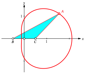
Fig. 6: B and C fix
For x = 0 we find the equilateral triangle (Fig. 7).
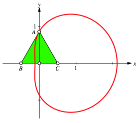
Fig. 7: Equilateral triangle
Note that the side AB of the equilateral triangle is tangential to the curve. For the proof we use the gradient:

The
vector ![]() is orthogonal to
the curve, but also orthogonal to the side AB
of the equilateral triangle.
is orthogonal to
the curve, but also orthogonal to the side AB
of the equilateral triangle.
For ![]() we get the large
Right Golden triangle (Fig. 8).
we get the large
Right Golden triangle (Fig. 8).
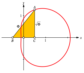
Fig. 8: Right Golden Triangle
We find
also the small Right Golden Triangle (Fig. 9). Here we have ![]()
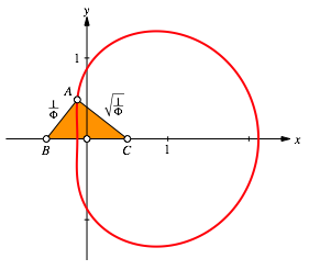
Fig. 9: Right Golden Triangle
Finally we find the Golden Section in different cases (Fig. 10 and 11). The major is indicated in blue and the minor in red.
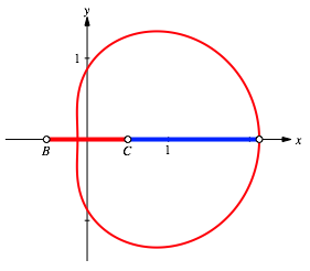
Fig. 10: Golden Section
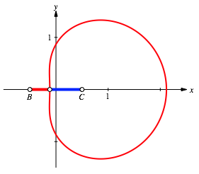
Fig. 11: Golden Section
3.2.2 C and A fix
Now we
choose ![]() and
and ![]() (Fig. 12).
(Fig. 12).
For the sides of the triangle we get:

The geometric sequence condition is again:
![]()
This yields the implicit equation for the locus of B:
![]()
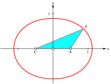
Fig. 12: C and A fix
The curve looks like an ellipse, but this cannot be, since it is a curve of degree 4. Nevertheless the difference to the ellipse with the same semi axes is very small (Fig. 13).
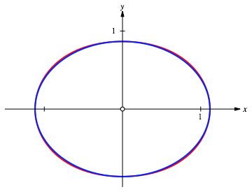
Fig. 13: Curve compared with ellipse
Again we find an equilateral triangle (Fig. 14), Right Golden triangles (Fig. 15) and the golden Section (Fig. 16).
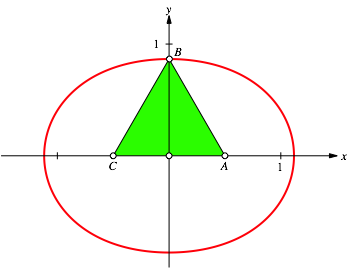
Fig. 14: Equilateral triangle
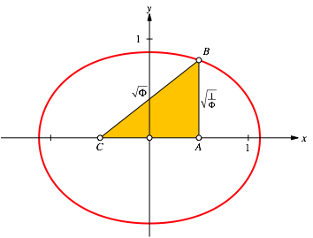
Fig. 15: Right Golden Triangle
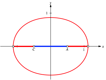
Fig. 16: Golden Section
3.2.3 A and B fix
Now we
choose ![]() and
and ![]() (Fig. 17).
(Fig. 17).
For the sides of the triangle we get:

The geometric sequence condition is again:
![]()
This yields the implicit equation for the locus of C:

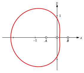
Fig. 17: A and B fix
The curve is symmetric to the curve of Figure 6.
3.3 The three curves
Figure 18 shows the three curves in a triangular lattice. We see a lot of Golden Sections.
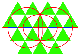
Fig. 18: The tree curves
References
Walser, Hans (2001): The Golden Section. Translated by Peter Hilton and Jean Pedersen. The Mathematical Association of America 2001. ISBN 0-88385-534-8.
Walser, Hans (6. Auflage). (2013). Der Goldene Schnitt. Mit einem Beitrag von Hans Wußing über populärwissenschaftliche Mathematikliteratur aus Leipzig. Leipzig: Edition am Gutenbergplatz. ISBN 978-3-937219-85-1.